13 Week 7 Demo
13.1 Setup
First, we’ll load the packages we’ll be using in this week’s brief demo. here we are pre-loading an already-estimated PMI matrix and results from the singular value decomposition approach.
# we need to install some of these packages from source
library(Matrix)
library(tidyverse)
library(tidytext)
library(umap) # for dimensionality reduction
library(quanteda)
library(RSpectra) # for singular value decompositionHow does it work?
- Various approaches, including:
- Singular value decomposition (SVD) - a dimensionality reduction technique, but not as semantically sophisticated as the neural network-based techniques
- Neural network-based techniques like GloVe and Word2Vec
In both approaches, we are:
- Defining a context window (see figure below)
- Looking at probabilities of word appearing near another words
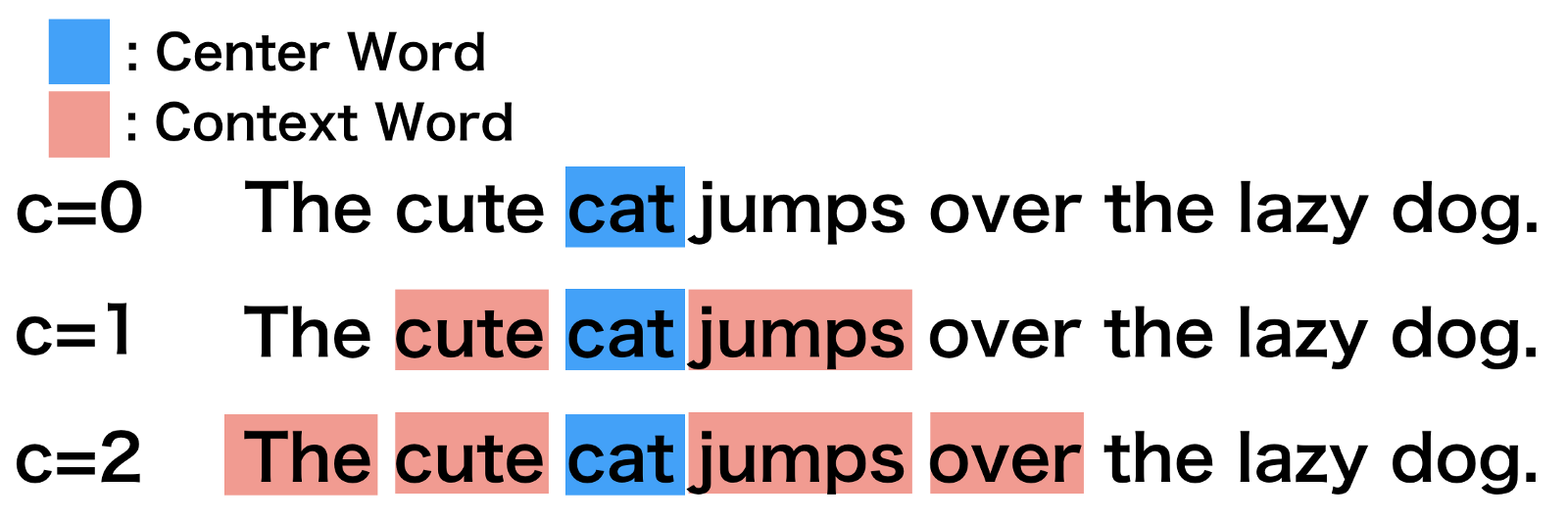
The implementation of this technique using the singular value decomposition approach requires the following data structure:
- Word pair matrix with PMI (Pairwise mutual information)
- where PMI = log(P(x,y)/P(x)P(y))
- and P(x,y) is the probability of word x appearing within a six-word window of word y
- and P(x) is the probability of word x appearing in the whole corpus
- and P(y) is the probability of word y appearing in the whole corpus
## 6 x 6 sparse Matrix of class "dgCMatrix"
##                the          to          and          of      https           a
## the    0.653259169 -0.01948121 -0.006446459  0.27136395 -0.5246159 -0.32557524
## to    -0.019481205  0.75498084 -0.065170433 -0.25694210 -0.5731182 -0.04595798
## and   -0.006446459 -0.06517043  1.027782342 -0.03974904 -0.4915159 -0.05862969
## of     0.271363948 -0.25694210 -0.039749043  1.02111517 -0.5045067  0.09829389
## https -0.524615878 -0.57311817 -0.491515918 -0.50450674  0.5451841 -0.57956404
## a     -0.325575239 -0.04595798 -0.058629689  0.09829389 -0.5795640  1.03048355
And the resulting matrix object will take the following format:
## Formal class 'dgCMatrix' [package "Matrix"] with 6 slots
##   ..@ i       : int [1:350700] 0 1 2 3 4 5 6 7 8 9 ...
##   ..@ p       : int [1:21173] 0 7819 14360 20175 25467 29910 34368 39207 43376 46401 ...
##   ..@ Dim     : int [1:2] 21172 21172
##   ..@ Dimnames:List of 2
##   .. ..$ : chr [1:21172] "the" "to" "and" "of" ...
##   .. ..$ : chr [1:21172] "the" "to" "and" "of" ...
##   ..@ x       : num [1:350700] 0.65326 -0.01948 -0.00645 0.27136 -0.52462 ...
##   ..@ factors : list()
We will then use the “Singular Value Decomposition” (SVD) techique. This is another multidimensional scaling technique, where the first axis of the resulting coordinates captures the most variance, the second the second-most etc…
And to do this, we simply need to do the following.
pmi_svd <- svds(pmi_matrix, 256)After which we can collect our vectors for each word and inspect them.
## [1] 21172 256
head(word_vectors[1:5, 1:5])## [,1] [,2] [,3] [,4] [,5]
## the 0.007810973 0.07024009 -0.06377615 0.03139044 0.12362108
## to 0.006889381 -0.03210269 -0.10665925 0.03537632 -0.10104552
## and -0.050498380 0.09131495 -0.19658197 -0.08136253 0.01605705
## of -0.015628371 0.16306386 -0.13296127 -0.04087709 0.23175976
## https 0.301718525 0.07658843 0.01720398 0.26219147 -0.07930941
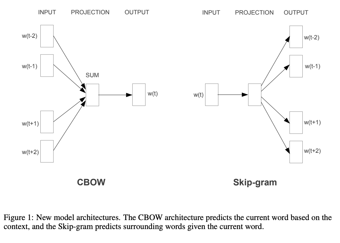
13.2 Using GloVe or word2vec
The neural network approach is considerably more involved, and the figure below gives an overview picture of the differing algorithmic approaches we might use.
13.3 Now with the Royals
This is text data from the Court circular (Pagnini). This original data has been collected by Marta Pagnini, who is a researcher at the London School of Economics. Each line is a paragraph in an issue of the Court Circular. The Court Circular is the official agenda of activities for the Royal family paper. It has been published every single day since the 19th century, giving information on what the Royals are doing and who they are meeting with.
court_circular <- read.csv2("data/wordembed/Court_Circular_1000_random_sample.csv", sep = ",")
head(court_circular)
## X Date
## 1 1 28 July 2007
## 2 2 13 July 2000
## 3 3 13 March 2012
## 4 4 30 June 2020
## 5 5 22 May 2006
## 6 6 12 April 2007
## Paragraph
## 1 Prince William of Wales today attended the World Scout Jamboree at Hylands Park, Chelmsford, and was received by Her Majesty's Lord-Lieutenant of Essex (the Lord Petre).
## 2 The Princess Royal, President of the Patrons, this morning visited Crime Concern's Youth Works Project, Preston Road Regeneration Centre, Flinton Grove, Kingston upon Hull, and was received by Her Majesty's Lord-Lieutenant of the East Riding of Yorkshire (Mr. Richard Marriott). Her Royal Highness, President of the Patrons, Crime Concern, later attended a seminar at BP Amoco Sports and Leisure Club, Saltend, Hedon, East Riding of Yorkshire. The Princess Royal, Patron, the National Autistic Society, this afternoon attended a Lunch at Sickling Hall, Sicklinghall Village, Wetherby, and was received by Mrs. Judith Thomas (Deputy Lieutenant of North Yorkshire). Her Royal Highness, Patron, the National Autistic Society, later opened the Robert Ogden School, Clayton Lane, Thurnscoe, Rotherham, and was received by Her Majesty's Lord-Lieutenant of South Yorkshire (the Earl of Scarbrough).
## 3 The Duchess of Gloucester this afternoon visited Lady Eleanor Holles School, Hanworth Road, Hampton, Middlesex, and unveiled a stone plaque to commemorate its Three Hundredth Anniversary, and was received by Her Majesty's Lord-Lieutenant of Greater London (Sir David Brewer).
## 4 The Earl and Countess of Wessex this morning visited Salute the NHS, Hangar 113, Bicester Motion, Skimmingdish Lane, Bicester, Oxfordshire. His Royal Highness this evening attended a Surrey Heath Prepared Meeting via video link. The Countess of Wessex this afternoon held a Meeting with the Lord Hague of Richmond (Co-Founder, Preventing Sexual Violence in Conflict Initiative) via video link. Her Royal Highness, Patron, Brendoncare Foundation, later held a Meeting via video link with Mrs. Carole Sawyers upon relinquishing her appointment as Chief Executive Officer and Mrs. Marianne Wanstall upon assuming the appointment.
## 5 The Princess Royal, Patron, RYA Sailability, this morning visited Colne Valley Special Sailors, the Aquadrome, Rickmansworth, and was received by Miss Linda Haye (Deputy Lieutenant of Hertfordshire). Her Royal Highness this afternoon visited Building Research Establishment Certification, Bucknalls Lane, Garston, Watford, and was received by Lady Staughton (Deputy Lieutenant of Hertfordshire). The Princess Royal, Patron, Sense - the National Deafblind and Rubella Association, later re-opened buildings at the Anne Wall Centre, 12 Hyde Close, Barnet, and was received by Mr. Stephen Folkes (Deputy Lieutenant of Greater London). Her Royal Highness this evening visited the Royal Horticultural Society's Chelsea Flower Show at the Royal Hospital Chelsea, London SW3. The Princess Royal, President, International League for the Protection of Horses, was represented by Mrs. Timothy Holderness-Roddam at the Service of Thanksgiving for Mrs. Vivien McIrvine (Past Vice President) which was held in the Guards Chapel, Wellington Barracks, Birdcage Walk, London SW1, today.
## 6 Princess Alexandra this afternoon opened the Michael Letcher Pathology Complex at the Princess Alexandra Hospital NHS Trust, Hamstel Road, Harlow, and was received by Her Majesty's Lord-Lieutenant of Essex (the Lord Petre).
# If you're working on your own computer, you can download the data directly from the course website repository
court_circular <- read.csv2(gzcon(url("https://github.com/marionlieutaud/CTA-ED/blob/main/data/wordembed/Court_Circular_1000_random_sample.csv?raw=true")), sep=",")
# There is a problem there
13.4 Word vectors via SVD
We’re going to set about generating a set of word vectors with from our court circular text data. Note that many word embedding applications will use pre-trained embeddings from a much larger corpus, or will generate local embeddings using neural net-based approaches.
Here, we’re instead going to generate a set of embeddings or word vectors by making a series of calculations based on the frequencies with which words appear in different contexts. We will then use a technique called the “Singular Value Decomposition” (SVD). This is a dimensionality reduction technique where the first axis of the resulting composition is designed to capture the most variance, the second the second-most etc…
How do we achieve this?
13.5 Implementation
The first thing we need to do is to get our data in the right format to calculate so-called “skip-gram probabilties.” If you go through the code line by the line in the below you will begin to understand what these are.
What’s going on?
Well, we’re first unnesting our tweet data as in previous exercises. But importantly, here, we’re not unnesting to individual tokens but to ngrams of length 6 or, in other words, for postID n with words k indexed by i, we take words i1 …i6, then we take words i2 …i7. Try just running the first two lines of the code below to see what this means in practice.
After this, we make a unique ID for the particular ngram we create for each postID, and then we make a unique skipgramID for each postID and ngram. And then we unnest the words of each ngram associated with each skipgramID.
You can see the resulting output below.
names(court_circular)## [1] "X" "Date" "Paragraph"
#create context window with length 6
court_skipgrams <- court_circular %>%
    rename(textID = X) %>%
    unnest_tokens(ngram, Paragraph, token = "ngrams", n = 6) %>%
    mutate(ngramID = row_number()) %>%
    tidyr::unite(skipgramID, textID, ngramID) %>%
    unnest_tokens(word, ngram)

head(court_skipgrams, n=20)
## skipgramID Date word
## 1 1_1 28 July 2007 prince
## 2 1_1 28 July 2007 william
## 3 1_1 28 July 2007 of
## 4 1_1 28 July 2007 wales
## 5 1_1 28 July 2007 today
## 6 1_1 28 July 2007 attended
## 7 1_2 28 July 2007 william
## 8 1_2 28 July 2007 of
## 9 1_2 28 July 2007 wales
## 10 1_2 28 July 2007 today
## 11 1_2 28 July 2007 attended
## 12 1_2 28 July 2007 the
## 13 1_3 28 July 2007 of
## 14 1_3 28 July 2007 wales
## 15 1_3 28 July 2007 today
## 16 1_3 28 July 2007 attended
## 17 1_3 28 July 2007 the
## 18 1_3 28 July 2007 world
## 19 1_4 28 July 2007 wales
## 20 1_4 28 July 2007 todayWhat next?
Well we can now calculate a set of probabilities from our skipgrams. We do so with the pairwise_count() function from the widyr package. Essentially, this function is saying: for each skipgramID count the number of times a word appears with another word for that feature (where the feature is the skipgramID). We set diag to TRUE when we also want to count the number of times a word appears near itself.
The probability we are then calculating is the number of times a word appears with another word denominated by the total number of word pairings across the whole corpus.
#package
library(widyr)

#calculate probabilities
skipgram_probs <- court_skipgrams %>%
    pairwise_count(word, skipgramID, diag = TRUE, sort = TRUE) %>% # diag = T means that we also count when the word appears twice within the window
    mutate(p = n / sum(n))

head(skipgram_probs[1000:1020,], n=20)
## # A tibble: 20 × 4
## item1 item2 n p
## <chr> <chr> <dbl> <dbl>
## 1 a later 231 0.0000980
## 2 later a 231 0.0000980
## 3 prince's prince's 231 0.0000980
## 4 north north 230 0.0000975
## 5 as relinquishing 230 0.0000975
## 6 relinquishing as 230 0.0000975
## 7 concert concert 230 0.0000975
## 8 great great 230 0.0000975
## 9 sir by 229 0.0000971
## 10 award this 229 0.0000971
## 11 excellency upon 229 0.0000971
## 12 duke patron 229 0.0000971
## 13 by sir 229 0.0000971
## 14 patron duke 229 0.0000971
## 15 this award 229 0.0000971
## 16 upon excellency 229 0.0000971
## 17 afternoon received 228 0.0000967
## 18 received afternoon 228 0.0000967
## 19 his to 228 0.0000967
## 20 to his 228 0.0000967## # A tibble: 20 × 4
## item1 item2 n p
## <chr> <chr> <dbl> <dbl>
## 1 a later 231 0.0000980
## 2 later a 231 0.0000980
## 3 prince's prince's 231 0.0000980
## 4 north north 230 0.0000975
## 5 as relinquishing 230 0.0000975
## 6 relinquishing as 230 0.0000975
## 7 concert concert 230 0.0000975
## 8 great great 230 0.0000975
## 9 sir by 229 0.0000971
## 10 award this 229 0.0000971
## 11 excellency upon 229 0.0000971
## 12 duke patron 229 0.0000971
## 13 by sir 229 0.0000971
## 14 patron duke 229 0.0000971
## 15 this award 229 0.0000971
## 16 upon excellency 229 0.0000971
## 17 afternoon received 228 0.0000967
## 18 received afternoon 228 0.0000967
## 19 his to 228 0.0000967
## 20 to his 228 0.0000967So we see, for example, that the words “duke” and “patron” appear 229 times together. Denominating that by the total n of word pairings (or sum(skipgram_probs$n)), gives us our probability p.
Currently our word embeddings include a lot of stopwords - we could consider removing them.
Okay, now we have our skipgram probabilities we need to get our “unigram probabilities” in order to normalize the skipgram probabilities before applying the singular value decomposition.
What is a “unigram probability”? Well, this is just a technical way of saying: count up all the appearances of a given word in our corpus then divide that by the total number of words in our corpus. And we can do this as such:
#calculate unigram probabilities (used to normalize skipgram probabilities later)
unigram_probs <- court_circular %>%
    unnest_tokens(word, Paragraph) %>%
    count(word, sort = TRUE) %>%
    mutate(p = n / sum(n))
Finally, it’s time to normalize our skipgram probabilities.
We take our skipgram probabilities, we filter out word pairings that appear twenty times or less. We rename our words “item1” and “item2,” we merge in the unigram probabilities for both words.
And then we calculate the joint probability as the skipgram probability divided by the unigram probability for the first word in the pairing divided by the unigram probability for the second word in the pairing. This is equivalent to: P(x,y)/P(x)P(y).
In essence, the interpretation of this value is: “do events (words) x and y occur together more often than we would expect if they were independent”?
Once we’ve recovered these normalized probabilities, we can have a look at the joint probabilities for a given item, i.e., word.
Here, we look at the word “charity” and “duke” and look at those words with the highest value for “p_together.”
Higher values greater than 1 indicate that the words are more likely to appear close to each other; low values less than 1 indicate that they are unlikely to appear close to each other. This, in other words, gives an indication of the association of two words.
#normalize skipgram probabilities
normalized_prob <- skipgram_probs %>%
    filter(n > 20) %>% #filter out skipgrams with n <=20
    rename(word1 = item1, word2 = item2) %>%
    left_join(unigram_probs %>%
                  select(word1 = word, p1 = p),
              by = "word1") %>%
    left_join(unigram_probs %>%
                  select(word2 = word, p2 = p),
              by = "word2") %>%
    mutate(p_together = p / p1 / p2)

normalized_prob %>%
    filter(word1 == "charity") %>%
    arrange(-p_together)
## # A tibble: 3 × 7
## word1 word2 n p p1 p2 p_together
## <chr> <chr> <dbl> <dbl> <dbl> <dbl> <dbl>
## 1 charity charity 72 0.0000305 0.000165 0.000165 1122.
## 2 charity a 24 0.0000102 0.000165 0.0112 5.52
## 3 charity the 28 0.0000119 0.000165 0.0870 0.827## # A tibble: 72 × 7
## word1 word2 n p p1 p2 p_together
## <chr> <chr> <dbl> <dbl> <dbl> <dbl> <dbl>
## 1 duke duke 3707 0.00157 0.0116 0.0116 11.8
## 2 duke edinburgh's 468 0.000198 0.0116 0.00162 10.6
## 3 duke rothesay 149 0.0000632 0.0116 0.000591 9.25
## 4 duke trustee 266 0.000113 0.0116 0.00111 8.77
## 5 duke edinburgh 764 0.000324 0.0116 0.00348 8.06
## 6 duke charles 151 0.0000640 0.0116 0.000866 6.40
## 7 duke york 474 0.000201 0.0116 0.00272 6.39
## 8 duke kent 266 0.000113 0.0116 0.00181 5.38
## 9 duke award 304 0.000129 0.0116 0.00210 5.30
## 10 duke gloucester 402 0.000170 0.0116 0.00322 4.59
## # ℹ 62 more rowsUsing this normalized probabilities, we then calculate the PMI or “Pointwise Mutual Information” value, which is simply the log of the joint probability we calculated above.
Definition time: “PMI is logarithm of the probability of finding two words together, normalized for the probability of finding each of the words alone.”
We then cast our word pairs into a sparse matrix where values correspond to the PMI between two corresponding words.
pmi_matrix <- normalized_prob %>%
    mutate(pmi = log10(p_together)) %>%
    cast_sparse(word1, word2, pmi)

#remove missing data
pmi_matrix@x[is.na(pmi_matrix@x)] <- 0
#run SVD
# Singular value decomposition
# The irlba package had problem compiling on MAC OS so
# switched from command irlba::irlba() to RSpectra::svds()
pmi_svd <- svds(pmi_matrix, 256)
glimpse(pmi_matrix)
## Formal class 'dgCMatrix' [package "Matrix"] with 6 slots
## ..@ i : int [1:12487] 0 1 2 3 4 5 6 7 8 9 ...
## ..@ p : int [1:1468] 0 725 1221 1607 1801 2013 2260 2385 2499 2594 ...
## ..@ Dim : int [1:2] 1467 1467
## ..@ Dimnames:List of 2
## .. ..$ : chr [1:1467] "the" "of" "and" "this" ...
## .. ..$ : chr [1:1467] "the" "of" "and" "this" ...
## ..@ x : num [1:12487] 0.2227 0.0361 -0.1723 -0.1849 -0.1372 ...
## ..@ factors : list()